In 2011 I finished my diploma thesis in the research area of partial differential equations on the topic of cloaking via change of variables. Cloaking had become an area of intense research, beginning with two publications in Science issue 312 in 2006, see references. In this post, I’ll give a short introduction presenting the main ideas.
The term cloaking is based on the idea of a cloak of invisibility. This area of research studies the possibility to hide an object from external measurements (think for example of a CT scan, where an object is scanned with electromagnetic radiation). The problem of cloaking is closely related to the theory of inverse problems. While, when solving partial differential equations - for example Maxwell’s equations - one is interested in a solution given initial values, boundary conditions and material parameters, inverse problems study the possibility to reconstruct those parameters for a given equation, when a solution is know (measured). The mathematical results show that this is not possible in general.
Maxwell’s equations constitute the foundations of electrodynamics. In the time-harmonic case, where the electric field $\mathcal{E}$ and the magnetic field $\mathcal{H}$ are expected to be of the form
$$ \mathcal{E}(x,t) = E(x)e^{-i\omega t}, \ \mathcal{H}(x,t) = H(x)e^{-i\omega t} $$
Maxwell’s equations can be written as
$$ \nabla\times E = -i\omega\mu H, \ \ \nabla\times H = i\omega\epsilon E $$
Here, we also assume that there are no external electric currents or charges. In the case of TM- or TE-mode, where the electric or magnetic fields have only one non-zero component, one can ultimately model the fields using a scalar Helmholtz equation. This is done in my thesis, which is based on Cloaking via change of variables for the Helmholtz equation, Kohn et al. 2010.
Change of variables
A change of variables is a mapping $f\colon M\rightarrow N$ that is differentiable and which inverse is differentiable as well (this kind of mapping is called diffeomorphism), where $M$ and $N$ are (smooth) manifolds - we will assume $M, N \subset \mathbb{R}^{n}$ here. We will also assume that the determinant of the Jacobian matrix $df$ is positive, that is $f$ preserves orientation.
One can show that Maxwell’s equations are invariant under such a change of variables. This means, if $E$ and $H$ are solutions of Maxwell’s equations, then the fields $$ \tilde{E}(y) = (df^{\top})^{-1}E(x), \ \ \tilde{H}(y) = (df^{\top})^{-1}H(x),\ \ x = f^{-1}(y) $$ satisfy Maxwell’s equations in transformed coordinates $$ \tilde{\nabla}\times \tilde{E} = -i\omega\tilde{\mu} \tilde{H}, \ \ \tilde{\nabla}\times \tilde{H} = i\omega\tilde{\epsilon}\tilde{E} $$ with material parameters $$ \tilde{\epsilon} := \frac{df\cdot\epsilon\cdot df^{\top}}{\det(df)}, \ \tilde{\mu} := \frac{df\cdot\mu\cdot df^{\top}}{\det(df)} $$
The invariance of Maxwell’s equations under changes of coordinates is the main ingredient to our cloaking approach, as we will explore in the next section.
As an example for a variable transformation, let’s take a look at the following mapping:
$$ F: B_2(0)\setminus{0} \rightarrow B_2(0)\setminus\overline{B_1(0)},\ \ F(x) = \left(1+\frac{1}{2}|x| \right)\frac{x}{|x|} $$
Notice that there is a singularity at $0$. The mapping expands this singularity to a ball with radius 1, while $F(x) = x$ at the outer boundary $|x|=2$. Most research papers on the topic will use this mapping (or variations) both for theoretical and numerical results.
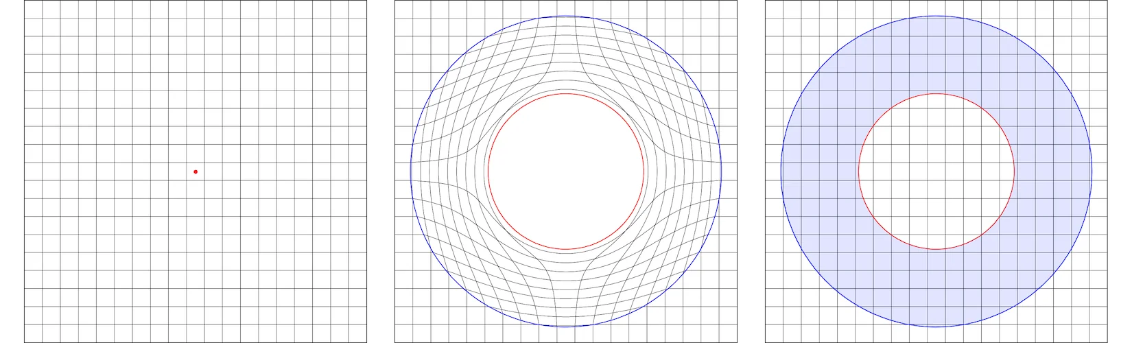
The image above shows the original region on the left and the transformed region in the middle. For the right image, consider the shaded region to be the cloak with material parameters given by above transformation. The outer region is free space and the inner region $|x|<1$ is the cloaked region, where material parameters can be arbitrary.
Cloaking
Let’s define how the term invisibility should be understood, i.e. which kind of measurement method will be used. Consider a sufficiently large area of space, which completely contains the object and the cloak surrounding the object. The measurements take place exclusively at the boundary of this area. An object can be considered invisible if the result of the measurement looks the same as the measurement of empty space.
-
Consider a wave propagating in empty space, i.e. Maxwell’s equations with homogeneous, isotropic material parameters apply. If we change the material parameters in a small area of space (e.g. the inclusion of a ball $B_{\rho}(x)$ with a small radius $\rho$), will the effect on the propagation of the wave also be small?
-
If we find a transformation that transforms this small inclusion to a sufficiently large area of the space, so that the object that should be hidden is included in this area, can we construct the transformation in such a way that the boundary measurements remain unaffected?
The answer to the second question is yes and the math behind it is again related to the theory of inverse problems and the so called Dirichlet-to-Neumann map (DtN) of the Helmholtz equation. The Dirichlet-to-Neumann map is the mathematical realization of the above idea of relating boundary measurements to the interior of a domain. Due to the invariance of Maxwell’s equations under a change of variables and the way the transformation $F$ is constructed, the DtN map of the solution with cloaking material parameters applied cannot be distinguished from the DtN map of a solution in empty space.
The answer to the first question unfortunately is no due to possible resonant frequencies. A large part of the analysis in the paper by Kohn et al. 2010 is spend by constructing a second, damping layer around the cloak and proving its effectiveness.
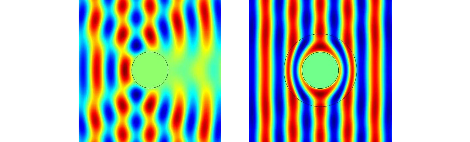
Theoretical results are confirmed by numerical simulations and also find applications in material science using metamaterials. The figure below on the left illustrates an analytic solution of the Helmholtz equation. An incoming plane wave with a frequency of 2 GHz (corresponds to a wave length of approx. 15 cm) is scattered from a perfectly conducting cylinder with a radius of 10 cm. The wave pattern shown is the sum of the incident field and the scattered field. The figure on the right shows the numerical simulation of a cloak computed with the finite element method.
References
-
Pendry et al. 2006
Pendry, J.B. ; D.Schurig ; Smith, D.R.: Controlling Electromagnetic Fields. In: Science 312 (2006), Nr. 5781, 1780-1782. https://doi.org/10.1126/science.1125907
-
Leonhardt 2006
Leonhardt, Ulf: Optical Conformal Mapping. In: Science 312 (2006), Nr. 5781, 1777-1780. https://dx.doi.org/10.1126/science.1126493
-
Cummer et al. 2006a
Cummer, Steven A. ; Schurig, David ; Smith, David R. ; Pendry, John: Fullwave simulations of electromagnetic cloaking structures. In: Physical Review E 74 (2006), Nr. 3, 036621. https://doi.org/10.48550/arXiv.physics/0607242
-
Cummer et al. 2006b
Cummer, Steven A. ; Schurig, David ; Smith, David R. ; Pendry, John: Metamaterial Electromagnetic Cloak at Microwave Frequencies. In: Science Express 314 (2006), Nr. 5801, 036621. https://doi.org/10.1126/science.1133628
-
Kohn et al. 2008
Kohn, R.V. ; Shen, H. ; Vogelius, M.S. ; Weinstein, M.I.: Cloaking via Change of Variables in Electric Impedance Tomography. In: Inverse Problems 24 (2008), Nr. 1, 015016. https://stacks.iop.org/0266-5611/24/i=1/a=015016
-
Kohn et al. 2010
Kohn, R.V. ; Onofrei, D. ; Vogelius, M.S. ; Weinstein, M.I.: Cloaking via change of variables for the Helmholtz equation. In: Communications on Pure and Applied Mathematics 63 (2010), 973-1016. https://doi.org/10.1002/cpa.20326
Please use the contact form for comments.